GIS Blog: Melanie A. Sutton

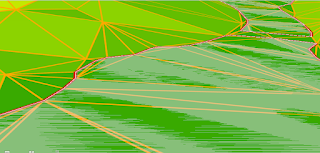
In this lab, we examined the effects of scale and resolution on the properties of spatial data. On vector data, as scale becomes finer, we expect to see increases in the number of areas and volumes, more detail in boundaries, and more homogeneity in the features (Goodchild, 2011, pp. 6). This occurs because coarser scales (e.g., 1:100000) are more generalized, and thus a smaller number of polygons capture the most significantly sized features, while omitting smaller features. As more details are captured at finer scales (e.g., 1:1200) compared to coarser scales, geometric characteristics such as the sum of total lengths for hydrographic features will increase, based on the addition of the captured smaller features. On raster data, as resolution becomes coarser (e.g., going from 1x1m to 90x90m cells), the image becomes more smoothed, as represented by increasingly smaller average slopes as steep regions are averaged into surrounding non-steep terrain regions. Kienzle observed this whe...

  In this lab we examined various interpolation methods to create a surface of water quality in Tampa Bay. Each method received as input a set of sample points containing Biochemical Oxygen Demand (BOD) values in milligrams per liter that were recorded from various points throughout the study region. The interpolation methods used this case study included the following: Thiessen IDW Spline - Regularized Spline - Tension This interpolation method is a special case of IDW where only the nearest water sample is used to estimate the BOD value at an unsampled location. This interpolation method uses a preset number of nearest neighbors to estimate the BOD value at an unsampled location, and inversely weights the contributing strength of these neighbors based on their distances from the unsampled location. Spline interpolation methods work to fit a smooth surface exactly touching the BOD sampled points, w...

Raster-based digital elevation models (DEMs) and vector-based triangulated irregular networks (TINs) are two alternative methods to represent digital topography. A DEM is sampled at a particular resolution and can only be made more accurate if the raster is resampled to a higher resolution. Alternatively, to make a TIN more accurate, additional points and breaklines can be added. For example, in the image below, to make the sharp boundaries around a lake more accurate, the TIN has been forced to use the exact boundaries and elevation of the lake polygon (shown in red): In the enhanced TIN above, notice how the TIN grid aligns perfectly along the shoreline with the addition of many more triangular cells in this area. Additionally, more triangles appear near the bends in the shoreline to more accurately capture these details. In this lab, we also learned how contour lines differ when derived from DEMs versus TINs. We observed that contour lines generated from a DEM are much smoother in...

  The goal of the accuracy assessment summarized in the map above was to determine quality of road networks provided by Jackson County GIS compared to a data set provided by the U.S. Census Bureau. One measure of such quality is the completeness of the data set, or how comprehensive the coverage of the data set is. As noted by Haklay (2010, pp. 690-692), one method to make this comparison between two data sets of road networks involves overlaying a grid over the study area and then calculating the difference in the total length of line segments in each cell. To get a percentage, one of the data sets serves as the base (in this case, the Jackson County GIS data set served this purpose). The calculated percentage can then be positive or negative based on this formula:      % difference = 100% * (Jackson County GIS - U.S. Census Bureau)/Jackson County GIS A positive value indicates better coverage by Jackson County GIS in the underlying grid cell (noted by shad...

  The image above shows 20 test point locations across a street map for the city of Albuquerque. In selecting these test points to report the horizontal accuracy of two alternative geographic data sources providing street centerlines, the following constraints were applied, in compliance with using the National Standard for Spatial Data Accuracy to measure and report the associated quality (Minnesota Planning Land Management Information Center, 2019): Locations were selected using street intersections derived from orthophotos of the study area - these images contained detailed imagery of street centerlines and nearby features (e.g., medians, sidewalks) that could be readily used to accurately determine intersection points. Given the street uniformity throughout the region, approximately 25% of the points were derived from each quadrant of the overall study area, and all quadrants were equally represented in this way (meeting the requirement to draw at least 20% of test points from ...

  Precision provides an assessment of the consistency of a measurement method (Bolstad, 2016, p. 624), or how close the measured values are to each other. The most commonly used measurement of precision is the distance that includes 68% of the repeated observations. For this dataset, as noted in the map legend above, the 68% horizontal precision value is 4.5 m. This means that 68% of independent observations are within 4.5 m of the average location. Alternatively, accuracy provides an assessment of how close a value is to the true value (Bolstad, 2016, p. 624). In this lab, horizontal accuracy was estimated as the distance between the average location and a known reference point, and was determined to be approximately 3.25 m.  With horizontal accuracy estimated as 3.25 m and 68% horizontal precision estimated as 4.5 m, we note a significant difference of 1.25 m between these values. Using a 68% horizontal precision value estimate means there are still 32% of the observations t...