Lab 6 [GIS5935]: Scale Effect and Spatial Data Aggregation
In this lab, we examined the effects of scale and resolution on the properties of spatial data. On vector data, as scale becomes finer, we expect to see increases in the number of areas and volumes, more detail in boundaries, and more homogeneity in the features (Goodchild, 2011, pp. 6). This occurs because coarser scales (e.g., 1:100000) are more generalized, and thus a smaller number of polygons capture the most significantly sized features, while omitting smaller features. As more details are captured at finer scales (e.g., 1:1200) compared to coarser scales, geometric characteristics such as the sum of total lengths for hydrographic features will increase, based on the addition of the captured smaller features.
On raster data, as resolution
becomes coarser (e.g., going from 1x1m to 90x90m cells), the image becomes more
smoothed, as represented by increasingly smaller average slopes as steep regions
are averaged into surrounding non-steep terrain regions. Kienzle observed this when
studying geomorphological features at cell sizes of 50, 100, and 250 m and noted
mean slope values decreased as the grid cell size increased (Kienzle, 2004, pp.
86). In addition, it was observed in this work that greater cell sizes caused greater
underestimations of slope (Kienzle, 2004, pp. 94). The larger impacts of this
for professional practice are that we should pay particular attention to scale
when using slope values to determine stability or erosion if the DEM is at a coarse
resolution, because the slope values are likely higher than estimates at this
scale indicate, particularly at resolutions greater than 2.5 m (Kienzle, 2004,
pp. 94).
In the second part of
the lab we studied spatial analyses related to gerrymandering, which is the
practice of manipulating the boundaries of polygons associated with districts for
unfair political advantage (Wikipedia, n.d.). Gerrymandering can be measured with
geoprocessing tools designed to mathematically capture a metric describing the
fairness of the polygon boundary capturing the district. One such metric is the
Polsby-Popper test for compactness, measured as:
(4.0*math.pi * !Shape_Area!) / (!Shape_Length! * !Shape_Length!)
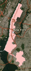
With this equation, the closer a Polsby-Popper value is to 1, the more compact (and thus fair) the polygon is. Here is a screenshot of an 'offending' district which fails to have district 'compactness' as measured by a Polsby-Popper value of 0.09:


Comments
Post a Comment