Lab 6 [GIS5007]: Isarithmic Mapping
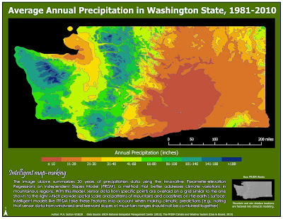
This week's lab focused on working with continuous raster data and exploring isarithmic mapping techniques that can be used to enhance the overall data visualization. Thematic maps based on continuous tone and hypsometric tinting were created, with the final map provided above created using ArcGIS Pro.
In
this final map, hypsometric tinting is implemented by manually classifying the
average annual precipitation values at each point into 10 classes, beginning
with ≤10 inches, 11-20 inches, and continuing through 141-180 inches, and
finally, >180 inches. The final shading began with red for the lowest values
and ramped up to deep blue for the higher values. Although it takes time to create the meaningful intervals for this type of visualization, this map demonstrates how symbolization based on hypsometric tinting is well-suited when you
want to display a more 3D-like image that reflects changes associated with
another phenomenon (in this case, changes in elevation). It is also a good choice here as it helps the viewer to more easily see
how a range of tints is associated to specific ranges of values for different locations on the map.
Another goal of this week's lab was to gain an appreciation for different interpolation methods used to create continuous raster data. The mapped precipitation data shown above was derived from
sensors over a 30-year window. Annual values of precipitation were derived from
monthly sums, and the 30-year average annual precipitation values for each
sensor were calculated from the average value of each sensor over the time
period of 1981-2010. The
innovative Parameter-elevation Regressions on Independent Slopes Model (PRISM) was then used to interpolate values between sensors while also intelligently addressing
known factors influencing climate variations (e.g., mountainous regions, rain
shadows, etc.).
With the PRISM interpolation model, sensor data from specific points are overlaid
on a grid similar to the one shown in the lower right inset map. This grid provides spatial scale and
patterns of mountains and coastlines on the earth's surface (e.g., grids may be
derived from digital elevation models, or DEMs). Intelligent models like PRISM take these
features into account when making climatic predictions (e.g., noting that
sensor data from windward and leeward slopes of mountain ranges should not be
combined together). In addition to location, elevation, coastal proximity,
topographic orientation, and topographic position, other factors considered
during the interpolation include vertical atmospheric layer and orthographic
effectiveness of the terrain.


Comments
Post a Comment